Model Registry Tutorials
Explore the full functionality of the Model Registry in this tutorial — from registering a model and inspecting its structure, to loading a specific model version for further use.
Model Registry
Throughout this tutorial we will leverage a local tracking server and model registry for simplicity. However, for production use cases we recommend using a remote tracking server.
Step 0: Install Dependencies
pip install --upgrade mlflow
Step 1: Register a Model
To use the MLflow model registry, you need to add your MLflow models to it. This is done through registering a given model via one of the below commands:
mlflow.<model_flavor>.log_model(registered_model_name=<model_name>): register the model while logging it to the tracking server.mlflow.register_model(<model_uri>, <model_name>): register the model after logging it to the tracking server. Note that you'll have to log the model before running this command to get a model URI.
MLflow has lots of model flavors. In the below example, we'll leverage scikit-learn's RandomForestRegressor to demonstrate the simplest way to register a model, but note that you can leverage any supported model flavor. In the code snippet below, we start an mlflow run and train a random forest model. We then log some relevant hyper-parameters, the model mean-squared-error (MSE), and finally log and register the model itself.
from sklearn.datasets import make_regression
from sklearn.ensemble import RandomForestRegressor
from sklearn.metrics import mean_squared_error
from sklearn.model_selection import train_test_split

import mlflow
import mlflow.sklearn

with mlflow.start_run() as run:
    X, y = make_regression(n_features=4, n_informative=2, random_state=0, shuffle=False)
    X_train, X_test, y_train, y_test = train_test_split(
        X, y, test_size=0.2, random_state=42
    )

    params = {"max_depth": 2, "random_state": 42}
    model = RandomForestRegressor(**params)
    model.fit(X_train, y_train)

    # Log parameters and metrics using the MLflow APIs
    mlflow.log_params(params)

    y_pred = model.predict(X_test)
    mlflow.log_metrics({"mse": mean_squared_error(y_test, y_pred)})

    # Log the sklearn model and register as version 1
    mlflow.sklearn.log_model(
        sk_model=model,
        name="sklearn-model",
        input_example=X_train,
        registered_model_name="sk-learn-random-forest-reg-model",
    )
Successfully registered model 'sk-learn-random-forest-reg-model'.
Created version '1' of model 'sk-learn-random-forest-reg-model'.
Great! We've registered a model.
Before moving on, let's highlight some important implementation notes.
- To register a model, you can leverage the
registered_model_nameparameter in themlflow.sklearn.log_model()or callmlflow.register_model()after logging the model. Generally, we suggest the former because it's more concise. - Model Signatures
provide validation for our model inputs and outputs. The
input_exampleinlog_model()automatically infers and logs a signature. Again, we suggest using this implementation because it's concise.
Explore the Registered Model
Now that we've logged an experiment and registered the model associated with that experiment run, let's observe how this information is actually stored both in the MLflow UI and in our local directory. Note that we can also get this information programmatically, but for explanatory purposes we'll use the MLflow UI.
Step 1: Explore the mlruns Directory
Given that we're using our local filesystem as our tracking server and model registry, let's observe the directory structure created when running the python script in the prior step.
Before diving in, it's import to note that MLflow is designed to abstract complexity from the user and this directory structure is just for illustration purposes. Furthermore, on remote deployments, which is recommended for production use cases, the tracking server will be on object store (S3, ADLS, GCS, etc.) and the model registry will be on a relational database (PostgreSQL, MySQL, etc.).
mlruns/
├── 0/                                    # Experiment ID
│   ├── bc6dc2a4f38d47b4b0c99d154bbc77ad/ # Run ID
│   │   ├── metrics/
│   │   │   └── mse                       # Example metric file for mean squared error
│   │   ├── artifacts/                    # Artifacts associated with our run
│   │   │   └── sklearn-model/
│   │   │       ├── python_env.yaml
│   │   │       ├── requirements.txt      # Python package requirements
│   │   │       ├── MLmodel               # MLflow model file with model metadata
│   │   │       ├── model.pkl             # Serialized model file
│   │   │       ├── input_example.json
│   │   │       └── conda.yaml
│   │   ├── tags/
│   │   │   ├── mlflow.user
│   │   │   ├── mlflow.source.git.commit
│   │   │   ├── mlflow.runName
│   │   │   ├── mlflow.source.name
│   │   │   ├── mlflow.log-model.history
│   │   │   └── mlflow.source.type
│   │   ├── params/
│   │   │   ├── max_depth
│   │   │   └── random_state
│   │   └── meta.yaml
│   └── meta.yaml
├── models/                               # Model Registry Directory
    ├── sk-learn-random-forest-reg-model/ # Registered model name
    │   ├── version-1/                    # Model version directory
    │   │   └── meta.yaml
    │   └── meta.yaml
The tracking server is organized by Experiment ID and Run ID and is responsible for storing our experiment artifacts, parameters, and metrics. The model registry, on the other hand, only stores metadata with pointers to our tracking server.
As you can see, flavors that support autologging provide lots of additional information out-of-the-box. Also note that even if we don't have autologging for our model of interest, we can easily store this information with explicit logging calls.
One more interesting callout is that by default you get three way to manage your model's
environment: python_env.yaml (python virtualenv), requirements.txt (PyPi requirements), and
conda.yaml (conda env).
Ok, now that we have a very high-level understanding of what is logged, let's use the MLflow UI to view this information.
Step 2: Start the Tracking Server
In the same directory as your mlruns folder, run the below command.
mlflow server --host 127.0.0.1 --port 8080
INFO:     Started server process [26393]
INFO:     Waiting for application startup.
INFO:     Application startup complete.
INFO:     Uvicorn running on http://127.0.0.1:8080 (Press CTRL+C to quit)
Step 3: View the Tracking Server
Assuming there are no errors, you can go to your web browser and visit http://localhost:8080 to
view the MLflow UI.
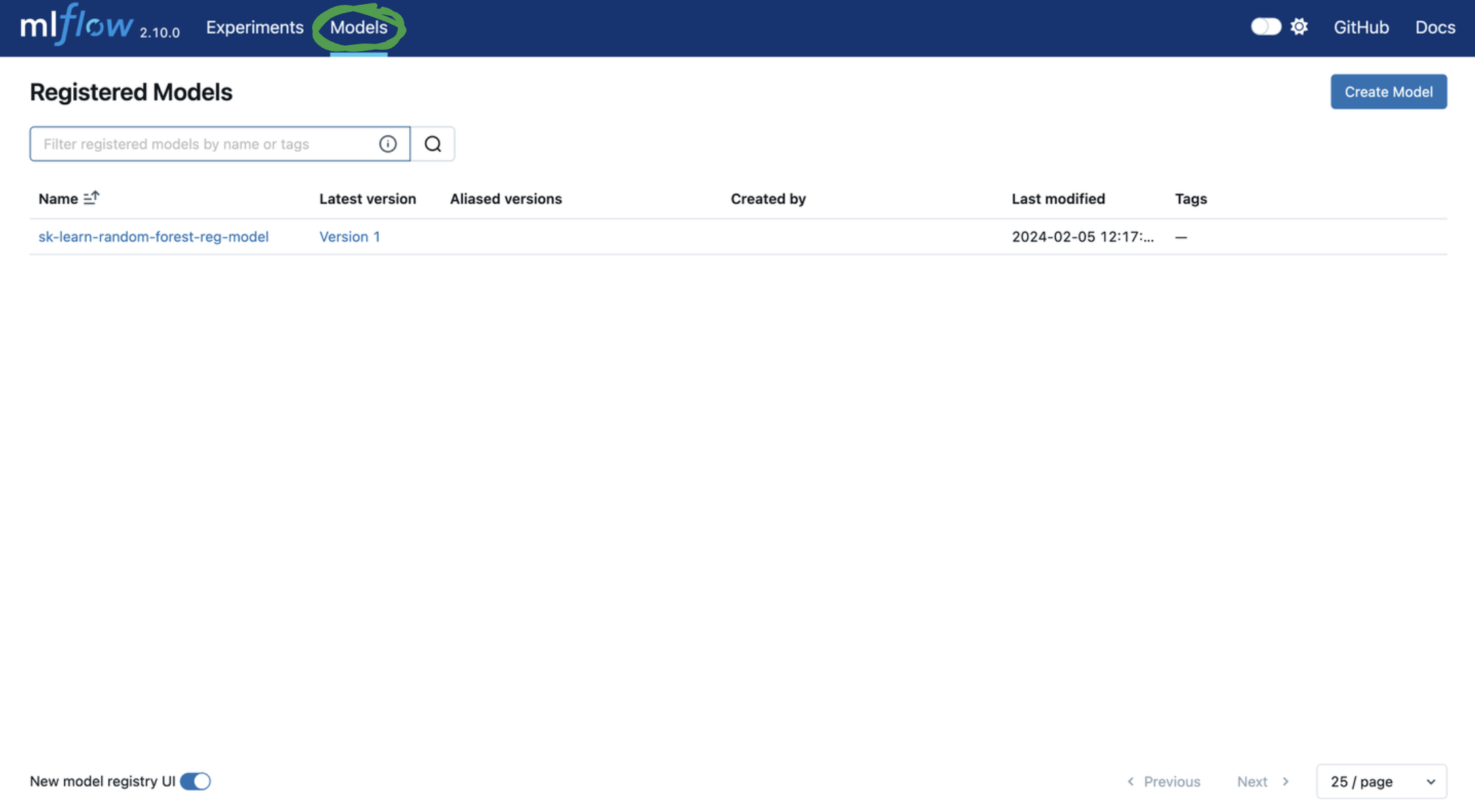
First, let's leave the experiment tracking tab and visit the model registry.
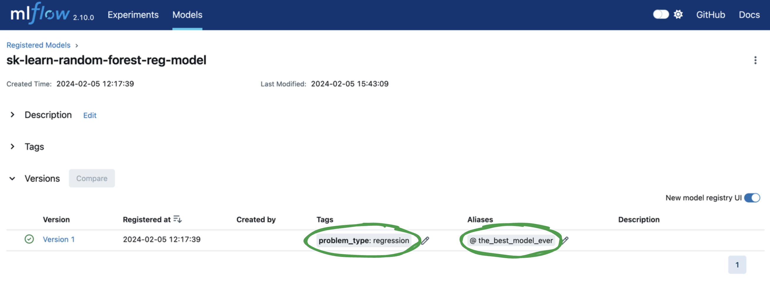
Next, let's add tags and a model version alias to
facilitate model deployment.
You can add or edit tags and aliases by clicking on the corresponding Add link or pencil icon in
the model version table. Let's...
- Add a model version tag with a key of
problem_typeand value ofregression. - Add a model version alias of
the_best_model_ever.
Load a Registered Model
To perform inference on a registered model version, we need to load it into memory. There are many ways to find our model version, but the best method differs depending on the information you have available. However, in the spirit of a quickstart, the below code snippet shows the simplest way to load a model from the model registry via a specific model URI and perform inference.
import mlflow.sklearn
from sklearn.datasets import make_regression

model_name = "sk-learn-random-forest-reg-model"
model_version = "latest"

# Load the model from the Model Registry
model_uri = f"models:/{model_name}/{model_version}"
model = mlflow.sklearn.load_model(model_uri)

# Generate a new dataset for prediction and predict
X_new, _ = make_regression(n_features=4, n_informative=2, random_state=0, shuffle=False)
y_pred_new = model.predict(X_new)

print(y_pred_new)
Note that if you're not using sklearn, if your model flavor is supported, you should use the
specific model flavor load method e.g. mlflow.<flavor>.load_model(). If the model flavor is
not supported, you should leverage mlflow.pyfunc.load_model(). Throughout this tutorial
we leverage sklearn for demonstration purposes.
Example 0: Load via Tracking Server
A model URI is a unique identifier for a serialized model. Given the model artifact is stored with experiments in the tracking server, you can use the below model URIs to bypass the model registry and load the artifact into memory.
- Absolute local path:
mlflow.sklearn.load_model("/Users/me/path/to/local/model") - Relative local path:
mlflow.sklearn.load_model("relative/path/to/local/model") - Run id:
mlflow.sklearn.load_model(f"runs:/{mlflow_run_id}/{run_relative_path_to_model}")
However, unless you're in the same environment that you logged the model, you typically won't have the above information. Instead, you should load the model by leveraging the model's name and version.
Example 1: Load via Name and Version
To load a model into memory via the model_name and monotonically increasing model_version,
use the below method:
model = mlflow.sklearn.load_model(f"models:/{model_name}/{model_version}")
While this method is quick and easy, the monotonically increasing model version lacks flexibility. Often, it's more efficient to leverage a model version alias.
Example 2: Load via Model Version Alias
Model version aliases are user-defined identifiers for a model version. Given they're mutable after model registration, they decouple model versions from the code that uses them.
For instance, let's say we have a model version alias called production_model, corresponding to
a production model. When our team builds a better model that is ready for deployment, we don't have
to change our serving workload code. Instead, in MLflow we reassign the production_model alias
from the old model version to the new one. This can be done simply in the UI. In the API, we run
client.set_registered_model_alias with the same model name, alias name, and new model version
ID. It's that easy!
In the prior page, we added a model version alias to our model, but here's a programmatic example.
import mlflow.sklearn
from mlflow import MlflowClient

client = MlflowClient()

# Set model version alias
model_name = "sk-learn-random-forest-reg-model"
model_version_alias = "the_best_model_ever"
client.set_registered_model_alias(
    model_name, model_version_alias, "1"
)  # Duplicate of step in UI

# Get information about the model
model_info = client.get_model_version_by_alias(model_name, model_version_alias)
model_tags = model_info.tags
print(model_tags)

# Get the model version using a model URI
model_uri = f"models:/{model_name}@{model_version_alias}"
model = mlflow.sklearn.load_model(model_uri)

print(model)
{'problem_type': 'regression'}
RandomForestRegressor(max_depth=2, random_state=42)
Model version alias is highly dynamic and can correspond to anything that is meaningful for your
team. The most common example is a deployment state. For instance, let's say we have a champion
model in production but are developing challenger model that will hopefully out-perform our
production model. You can use champion and challenger model version aliases to uniquely
identify these model versions for easy access.
That's it! You should now be comfortable...
- Registering a model
- Finding a model and modifying the tags and model version alias via the MLflow UI
- Loading the registered model for inference